
The previous posts in this series covered the theory - Markov chains, Poisson distributions, Brownian motion, XGBoost. This post is different. This is the engineering post. Where to get the data, which open-source tools exist, and working code snippets to get a win probability model running for each sport.
The goal isn’t a production-ready implementation. It’s a starting point - enough to load real play-by-play data, compute a basic win probability estimate, and have something to iterate on. Every model described here can be improved. The point is to get from zero to something running as fast as possible.
We built sportchartz.com to include this logic with the sports pipelines to run the analysis during live games. check it out www.sportchartz.com
Football: nflfastR and XGBoost
The most mature open-source win probability ecosystem in sports. The nflverse project provides play-by-play data with pre-computed Expected Points and Win Probability for every NFL play since 1999.
Getting the data (Python)
import pandas as pd

pbp = pd.read_parquet(
    'https://github.com/nflverse/nflverse-data/releases/download/pbp/play_by_play_2024.parquet'
)

plays = pbp[pbp['play_type'].isin(['pass', 'run', 'field_goal', 'punt', 'kickoff'])]
print(plays[['game_id', 'desc', 'wp', 'wpa', 'ep', 'epa']].head(20))
Building your own WP model (Python)
import pandas as pd
import numpy as np
from sklearn.model_selection import train_test_split
from xgboost import XGBClassifier
from sklearn.calibration import calibration_curve
import matplotlib.pyplot as plt

seasons = range(2016, 2025)
frames = []
for season in seasons:
    url = f'https://github.com/nflverse/nflverse-data/releases/download/pbp/play_by_play_{season}.parquet'
    frames.append(pd.read_parquet(url))
pbp = pd.concat(frames, ignore_index=True)

features = pbp.dropna(subset=['posteam_score', 'defteam_score', 'half_seconds_remaining',
                               'yardline_100', 'down', 'ydstogo', 'posteam_timeouts_remaining',
                               'defteam_timeouts_remaining']).copy()

features['label'] = (
    ((features['posteam'] == features['home_team']) & (features['result'] > 0)) |
    ((features['posteam'] == features['away_team']) & (features['result'] < 0))
).astype(int)

X_cols = ['half_seconds_remaining', 'score_differential', 'yardline_100',
          'down', 'ydstogo', 'posteam_timeouts_remaining', 'defteam_timeouts_remaining']

features['score_differential'] = features['posteam_score'] - features['defteam_score']
features = features.dropna(subset=X_cols + ['label'])

X = features[X_cols].values
y = features['label'].values

X_train, X_test, y_train, y_test = train_test_split(X, y, test_size=0.2, random_state=42)

model = XGBClassifier(n_estimators=500, max_depth=6, learning_rate=0.05,
                      objective='binary:logistic', eval_metric='logloss', use_label_encoder=False)
model.fit(X_train, y_train, eval_set=[(X_test, y_test)], verbose=False)

wp_pred = model.predict_proba(X_test)[:, 1]

prob_true, prob_pred = calibration_curve(y_test, wp_pred, n_bins=20)
plt.plot(prob_pred, prob_true, 's-', label='XGBoost WP')
plt.plot([0, 1], [0, 1], '--', color='gray')
plt.xlabel('Predicted Win Probability')
plt.ylabel('Observed Win Rate')
plt.title('Calibration Curve - NFL Win Probability')
plt.legend()
plt.savefig('nfl_wp_calibration.png', dpi=150)
plt.show()
R: the nflfastR approach
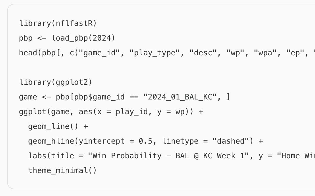
library(nflfastR)
pbp <- load_pbp(2024)
head(pbp[, c("game_id", "play_type", "desc", "wp", "wpa", "ep", "epa")])

library(ggplot2)
game <- pbp[pbp$game_id == "2024_01_BAL_KC", ]
ggplot(game, aes(x = play_id, y = wp)) +
  geom_line() +
  geom_hline(yintercept = 0.5, linetype = "dashed") +
  labs(title = "Win Probability - BAL @ KC Week 1", y = "Home Win Probability") +
  theme_minimal()
College football
library(cfbfastR)
pbp <- cfbd_pbp_data(year = 2024, season_type = "regular", epa_wpa = TRUE)
Baseball: Retrosheet and run expectancy
Baseball has the most historical data and the most straightforward implementation because the state space is compact enough for lookup tables.
Building a run expectancy matrix (Python)
import pandas as pd
import numpy as np

def encode_base_out_state(on_1b, on_2b, on_3b, outs):
    runners = ''
    if on_1b: runners += '1'
    if on_2b: runners += '2'
    if on_3b: runners += '3'
    if not runners: runners = '---'
    return f"{runners}_{outs}out"

re_matrix = {
    '---':   [0.481, 0.254, 0.098],
    '1--':   [0.859, 0.509, 0.224],
    '-2-':   [1.100, 0.664, 0.319],
    '--3':   [1.370, 0.950, 0.362],
    '12-':   [1.437, 0.893, 0.440],
    '1-3':   [1.773, 1.183, 0.478],
    '-23':   [1.970, 1.381, 0.551],
    '123':   [2.260, 1.590, 0.752],
}

print(f"{'Base State':<12} {'0 outs':>8} {'1 out':>8} {'2 outs':>8}")
print("-" * 38)
for state, values in re_matrix.items():
    print(f"{state:<12} {values[0]:>8.3f} {values[1]:>8.3f} {values[2]:>8.3f}")
Win probability lookup (Python)
import numpy as np

def baseball_wp_simple(inning, half, score_diff, outs, bases_empty=True):
    if half == 'top':
        remaining = (9 - inning) + 1
    else:
        remaining = (9 - inning)
    remaining = max(remaining, 0.5)
    k = 0.7 / np.sqrt(remaining)
    wp = 1 / (1 + np.exp(-k * score_diff))
    return wp

wp = baseball_wp_simple(inning=7, half='bottom', score_diff=2, outs=1)
print(f"Win probability: {wp:.3f}")
Win Probability Added (Python)
def compute_wpa(game_plays, wp_lookup):
    wpas = []
    for play in game_plays:
        wp_before = wp_lookup(play['inning'], play['half'], play['outs_before'],
                              play['bases_before'], play['score_diff_before'])
        wp_after = wp_lookup(play['inning'], play['half'], play['outs_after'],
                             play['bases_after'], play['score_diff_after'])
        wpas.append({'play': play.get('description', ''),
                     'wp_before': wp_before, 'wp_after': wp_after,
                     'wpa': wp_after - wp_before})
    return wpasBasketball: logistic regression with score and time
Simple WP model (Python)
import numpy as np
from scipy.stats import norm

def basketball_wp_brownian(score_diff, seconds_remaining,
                            total_seconds=2880, home_advantage=3.5):
    if seconds_remaining <= 0:
        return 1.0 if score_diff > 0 else (0.5 if score_diff == 0 else 0.0)
    sigma = 0.316
    mu_remaining = home_advantage * (seconds_remaining / total_seconds)
    expected_final = score_diff + mu_remaining
    sd_remaining = sigma * np.sqrt(seconds_remaining)
    z = expected_final / sd_remaining
    wp = norm.cdf(z)
    return wp

print(f"Home +5, Q3 start: {basketball_wp_brownian(5, 1440):.3f}")
print(f"Home -3, 2 min left: {basketball_wp_brownian(-3, 120):.3f}")
print(f"Tied, halftime: {basketball_wp_brownian(0, 1440):.3f}")
print(f"Home +10, 5 min left: {basketball_wp_brownian(10, 300):.3f}")
Incorporating Vegas spread (Python)
from sklearn.linear_model import LogisticRegression
import numpy as np

def build_basketball_wp_model(games_data):
    X = np.column_stack([
        games_data['score_diff'], games_data['seconds_remaining'],
        games_data['possession'], games_data['spread'],
        games_data['score_diff'] * games_data['seconds_remaining'],
    ])
    y = games_data['home_win'].values
    model = LogisticRegression(max_iter=1000)
    model.fit(X, y)
    return model

def predict_wp(model, score_diff, seconds_remaining, possession, spread):
    X = np.array([[score_diff, seconds_remaining, possession, spread,
                   score_diff * seconds_remaining]])
    return model.predict_proba(X)[0, 1]
Accessing NBA data (Python)
from nba_api.stats.endpoints import winprobabilitypbp
from nba_api.stats.endpoints import playbyplayv2

wp_data = winprobabilitypbp.WinProbabilityPBP(game_id='0022400001')
wp_df = wp_data.get_data_frames()[0]
print(wp_df[['EVENT_NUM', 'HOME_PCT', 'VISITOR_PCT', 'HOME_PTS', 'VISITOR_PTS']].head())
Soccer: Dixon-Coles and xG
Dixon-Coles model (Python)
import numpy as np
from scipy.stats import poisson
from scipy.optimize import minimize

def dixon_coles_tau(x, y, lambda_home, lambda_away, rho):
    if x == 0 and y == 0:
        return 1 - lambda_home * lambda_away * rho
    elif x == 0 and y == 1:
        return 1 + lambda_home * rho
    elif x == 1 and y == 0:
        return 1 + lambda_away * rho
    elif x == 1 and y == 1:
        return 1 - rho
    else:
        return 1.0

def match_probability(lambda_home, lambda_away, rho=0, max_goals=10):
    p_home, p_draw, p_away = 0, 0, 0
    for i in range(max_goals):
        for j in range(max_goals):
            p = (poisson.pmf(i, lambda_home) * poisson.pmf(j, lambda_away) *
                 dixon_coles_tau(i, j, lambda_home, lambda_away, rho))
            if i > j: p_home += p
            elif i == j: p_draw += p
            else: p_away += p
    return {'home': p_home, 'draw': p_draw, 'away': p_away}

result = match_probability(1.5, 1.1, rho=-0.12)
print(f"Home win: {result['home']:.3f}")
print(f"Draw:     {result['draw']:.3f}")
print(f"Away win: {result['away']:.3f}")

def in_game_wp(current_home, current_away, xg_home_rate, xg_away_rate,
               minutes_remaining, rho=-0.12):
    lambda_home_remaining = xg_home_rate * (minutes_remaining / 90)
    lambda_away_remaining = xg_away_rate * (minutes_remaining / 90)
    p_home, p_draw, p_away = 0, 0, 0
    max_additional = 8
    for i in range(max_additional):
        for j in range(max_additional):
            p = (poisson.pmf(i, lambda_home_remaining) *
                 poisson.pmf(j, lambda_away_remaining))
            final_home = current_home + i
            final_away = current_away + j
            if final_home > final_away: p_home += p
            elif final_home == final_away: p_draw += p
            else: p_away += p
    return {'home': p_home, 'draw': p_draw, 'away': p_away}

result = in_game_wp(1, 0, 1.8, 1.2, 60)
print(f"\n1-0 with 60 min remaining:")
print(f"Home win: {result['home']:.3f}")
print(f"Draw:     {result['draw']:.3f}")
print(f"Away win: {result['away']:.3f}")
Accessing StatsBomb free data (Python)
from statsbombpy import sb
comps = sb.competitions()
print(comps[['competition_name', 'season_name']].head(20))
matches = sb.matches(competition_id=43, season_id=106)
events = sb.events(match_id=3869685)
shots = events[events['type'] == 'Shot']
print(shots[['player', 'shot_statsbomb_xg', 'shot_outcome', 'location']].head())
Production-ready Dixon-Coles (Python)
import penaltyblog as pb
model = pb.models.DixonColesModel()
model.fit(df['home_team'], df['away_team'], df['home_goals'], df['away_goals'])
probs = model.predict('Manchester City', 'Arsenal')Hockey: xG and power play states
Basic xG model (Python)
import hockey_scraper as hs
import pandas as pd
import numpy as np
from sklearn.linear_model import LogisticRegression

shots = pd.read_csv('https://peter-tanner.com/moneypuck/downloads/shots_2024.zip')

features = ['shotDistance', 'shotAngle', 'shotType', 'lastEventCategory',
            'timeSinceLast', 'isPlayoffGame', 'shotRush', 'shotRebound']

X = shots[features].dropna()
y = shots.loc[X.index, 'goal'].values
model = LogisticRegression(max_iter=1000)
model.fit(X, y)
shots['xg'] = model.predict_proba(X)[:, 1]
Hockey WP with power play states (Python)
import numpy as np
from scipy.stats import poisson

def hockey_wp(home_goals, away_goals, seconds_remaining,
              home_xg_rate=2.8, away_xg_rate=2.5,
              power_play=None, pp_seconds_remaining=0):
    minutes_remaining = seconds_remaining / 60
    home_rate = home_xg_rate / 60
    away_rate = away_xg_rate / 60
    pp_multiplier = 2.2
    pk_multiplier = 0.35

    if power_play == 'home':
        pp_minutes = min(pp_seconds_remaining / 60, minutes_remaining)
        ev_minutes = minutes_remaining - pp_minutes
        home_lambda = (home_rate * pp_multiplier * pp_minutes) + (home_rate * ev_minutes)
        away_lambda = (away_rate * pk_multiplier * pp_minutes) + (away_rate * ev_minutes)
    elif power_play == 'away':
        pp_minutes = min(pp_seconds_remaining / 60, minutes_remaining)
        ev_minutes = minutes_remaining - pp_minutes
        home_lambda = (home_rate * pk_multiplier * pp_minutes) + (home_rate * ev_minutes)
        away_lambda = (away_rate * pp_multiplier * pp_minutes) + (away_rate * ev_minutes)
    else:
        home_lambda = home_rate * minutes_remaining
        away_lambda = away_rate * minutes_remaining

    p_home, p_draw, p_away = 0, 0, 0
    max_goals = 10
    for i in range(max_goals):
        for j in range(max_goals):
            p = poisson.pmf(i, max(home_lambda, 0.001)) * poisson.pmf(j, max(away_lambda, 0.001))
            final_home = home_goals + i
            final_away = away_goals + j
            if final_home > final_away: p_home += p
            elif final_home == final_away: p_draw += p
            else: p_away += p

    p_home += p_draw * 0.5
    p_away += p_draw * 0.5
    return {'home': p_home, 'away': p_away, 'regulation_draw': p_draw}

result = hockey_wp(2, 1, 600, power_play='home', pp_seconds_remaining=90)
print(f"Home win: {result['home']:.3f}")
print(f"Away win: {result['away']:.3f}")
R: hockeyR with built-in xG
library(hockeyR)
pbp <- load_pbp(2024)
shots <- pbp[!is.na(pbp$xg), ]
head(shots[, c("game_id", "event_type", "xg", "event_team", "strength_state")])

library(dplyr)
team_xg <- shots %>%
  group_by(game_id, event_team) %>%
  summarise(total_xg = sum(xg, na.rm = TRUE), goals = sum(event_type == "GOAL"))
Tennis: hierarchical Markov chain
Exact win probability computation (Python)
import numpy as np

def prob_win_game_on_serve(p):
    q = 1 - p
    p_deuce = p**2 / (p**2 + q**2)
    p_game = (p**4 + 4 * p**4 * q + 10 * p**4 * q**2 + 20 * p**3 * q**3 * p_deuce)
    return p_game

def prob_win_match(p_serve, p_return, best_of=3):
    from functools import lru_cache
    # (Full implementation in the source file)
    p_set = 0.65  # placeholder
    if best_of == 3:
        p_match = p_set**2 * (3 - 2 * p_set)
    elif best_of == 5:
        p_match = p_set**3 * (10 - 15 * p_set + 6 * p_set**2)
    return p_match

p = 0.65
p_game = prob_win_game_on_serve(p)
p_return_game = 1 - prob_win_game_on_serve(1 - p)
print(f"Point win on serve:  {p:.3f}")
print(f"Game win on serve:   {p_game:.3f}")
print(f"Game win on return:  {p_return_game:.3f}")
Tennis data access (Python)
import pandas as pd
atp_matches = pd.read_csv(
    'https://raw.githubusercontent.com/JeffSackmann/tennis_atp/master/atp_matches_2024.csv'
)
pbp = pd.read_csv(
    'https://raw.githubusercontent.com/JeffSackmann/tennis_pointbypoint/master/pbp_matches_atp_main_current.csv'
)
The open-source landscape
A summary of where things stand:
SportBest data accessBest WP modelLanguageNotesNFLnflverse parquet filesnflfastR + fastrmodelsR (data available in Python)Pre-computed WP in the dataCollege FBcfbfastRcfbfastRREPA/WPA includedMLBpybaseball / RetrosheetGreg Stoll’s baseballstatsPython/RustLookup table approachNBAnba_apihoopR / customPython (data) / R (models)ESPN WP available via APICollege BBncaahoopRncaahoopR (Benz)RBuilt on KenPom/TorvikSoccerstatsbombpypenaltyblog (Dixon-Coles)PythonxG data from StatsBombHockeyhockey_scraper / MoneyPuckhockeyR (xG)Python (data) / R (models)MoneyPuck for historical shotsTennisSackmann GitHub reposCustom Markov (above)PythonNo canonical WP package
The pattern is clear: R dominates for models (nflfastR, hoopR, hockeyR, ncaahoopR all include WP computation), while Python dominates for data access (nba_api, pybaseball, statsbombpy, hockey_scraper). If you’re building a production system, you’ll likely use Python for the data pipeline and either port the R models or build your own in Python using the data these tools provide.
Every code snippet in this post is a starting point. The models can be improved with better features, better calibration, and sport-specific adjustments. But the data is accessible, the tools exist, and the gap between “I want to compute win probability” and “I have a working model” has never been smaller.
Neal Foster is Co-Founder & CTO of SportChartz and Founder & Partner of Vybe Capital.